[Paper review] Vector Compression Method for HNSW – Flash

Pangyoalto

Sep 1, 2025 • 15 min read

This post reviews the paper Accelerating Graph Indexing for ANNS on Modern CPUs.

To fully understand this paper, familiarity with HNSW and Product Quantization is helpful.

HNSW is the most widely used algorithm for vector search. Since the HNSW paper was published in 2016, it has now been in use for nearly a decade, and many follow-up papers have been released to optimize it.

The paper we’re covering this time, Accelerating Graph Indexing for ANNS on Modern CPUs, is a relatively recent work accepted at SIGMOD 2025.

What makes this paper different from previous HNSW optimization research is that it introduces a new technique—Flash—for compressing the vectors stored in the index. Earlier studies mostly focused on improving the HNSW algorithm itself or optimizing it to run better on specialized hardware like GPUs.

According to the paper, applying Flash to compress vectors speeds up indexing by 10–20× and reduces index size by 2–5× compared to standard HNSW indexing.

Flash does not require algorithmic modifications or special hardware, making it easy to adopt across many services. If you are working with vector search, you will likely find valuable insights by reading through this post.

Introduction: Why is Graph Indexing Still Slow on Modern CPUs?

When the number of vectors is small, indexing speed is not a problem. However, when the number of vectors reaches tens of millions to hundreds of millions, building an HNSW index alone can take several hours to tens of hours. Even if the index is rebuilt during off-peak hours at night, if the dataset exceeds 100 million vectors, the process may spill over into the next day, making it difficult to provide users with up-to-date search results.

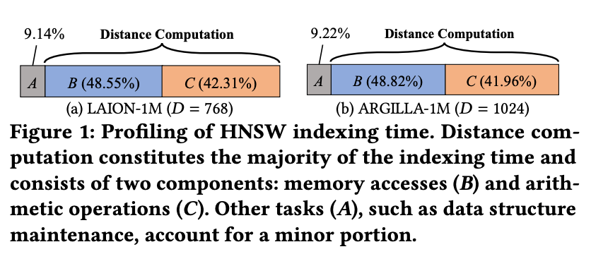
Accelerating Graph Indexing for ANNS on Modern CPUs

In the paper, the authors profiled the HNSW index construction process on real embedding datasets and found that about 90% of the total indexing time was spent on distance computations. Among this, memory access and arithmetic operations were almost evenly split.

The two biggest reasons are:

Random Memory Access: Vectors in an HNSW index have little spatial locality in memory. As a result, each distance computation requires fetching data from random locations, leading to frequent cache misses.
Reduced SIMD Efficiency: Most vectors are high-dimensional (e.g., 768 dimensions) and use 4-byte float values. For example, a 768-dimensional float vector occupies about 3KB of memory. Meanwhile, modern CPU SIMD instructions generally process data in 128-bit (SSE) or 256-bit (AVX) chunks, so computing with such vectors requires multiple memory loads and partial operations. This prevents SIMD from fully delivering its parallel performance potential.

Earlier, we mentioned prior research that attempted to accelerate HNSW using GPUs. However, the paper points out that GPUs also have significant limitations:

Cost: High-performance GPUs (e.g., NVIDIA A100) are expensive.
Memory Limitations: Even an A100 GPU, with its 10GB memory capacity, cannot handle embedding datasets that span hundreds of gigabytes.
Engineering Complexity: GPU acceleration requires specialized code for parallelization and ongoing maintenance.

For these practical reasons, most vector search systems still run on CPUs. However, with conventional methods, CPU-based indexing performance has clear limitations.

Problem Analysis – Distance Computation

Earlier, we saw that the bottleneck in HNSW index construction arises from distance computations. The paper further analyzes which parts of the distance computation process cause this bottleneck.

Notation

Each vector is denoted by bold lowercase letters such as x, y.
The Euclidean distance between two vectors is written as 𝛿(x, y).
Sets are denoted by bold uppercase letters such as X, C(x).

HNSW index construction can be divided into two main steps:

Candidate Acquisition (CA)
Neighbor Selection (NS)

Candidate Acquisition (CA)

CA is the process of finding candidate vectors that are close to a newly inserted vector. At this stage, HNSW performs a greedy search.

Since the graph stores only neighbor IDs (and not the vector values themselves), the actual vector data must be fetched from memory each time a distance computation is required. This results in random memory access.

Neighbor Selection (NS)

NS is the step where the algorithm selects actual neighbors from the candidates collected during CA. This involves computing distances between the candidates themselves, as well as comparing them again with the input vector. This process also triggers random memory access to fetch vector data.

In both CA and NS, random memory access occurs repeatedly. The resulting cache misses and memory latency significantly degrade performance.

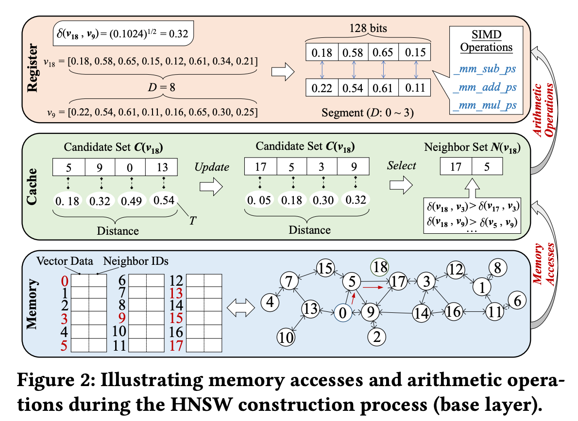
Let’s Walk Through an Example of Index Construction with Figure 2.

Figure 2 illustrates the process of inserting vector v₁₈ into the graph. In this example, the candidate set size C is 4, and the final number of neighbors R is 2.

Candidate Acquisition (CA)

When inserting v₁₈, the search starts from vector v₀.
By checking v₀’s neighbors and computing their distances, the initial candidate set is formed: C(v₁₈) = {v₅, v₉, v₀, v₁₃}.
The farthest distance, 𝛿(v₁₈, v₁₃) = 0.54, is set as the threshold T.
Next, the search moves to the closest neighbor, v₅, and examines its neighbors.
After computing distances among the new candidates, only those with distances smaller than T are kept and the candidate set is updated.
The final candidate set becomes: C(v₁₈) = {v₁₇, v₅, v₃, v₉}.

Neighbor Selection (NS)

The closest neighbor, v₁₇, is selected first.
Based on HNSW’s heuristic for finalizing candidates: Since 𝛿(v₁₇, v₃) < 𝛿(v₃, v₁₈) and 𝛿(v₁₇, v₉) < 𝛿(v₉, v₁₈), both v₃ and v₉ are eliminated.
As a result, v₅ and v₁₇ are finally connected to v₁₈.

Throughout the CA and NS steps, the accessed vectors are scattered randomly in memory. Looking at the memory layout at the bottom of Figure 2, we can see that the selected candidates are located far apart from each other. This leads to repeated cache misses during the process.

Can We Still Compare Distances Accurately After Vector Compression?

This paper designs a new compression method based on existing techniques such as PQ (Product Quantization), SQ (Scalar Quantization), and PCA (Principal Component Analysis).

To apply vector compression, the crucial requirement is that the results of distance comparisons using compressed vectors must remain consistent with those using the original vectors.

Distance Comparison After Compression

The paper breaks down the distance computations in HNSW indexing into two categories:

DC1: Distance calculations when updating candidates
DC2: Distance calculations when selecting final neighbors

It then presents the necessary conditions under which the comparison of distances between a newly inserted vector u and existing vectors v and w will yield the same result even after compression.

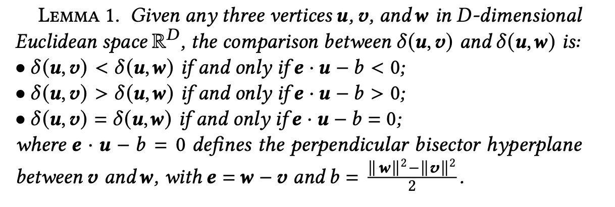
The paper introduces an alternative method for distance comparison through Lemma 1 (see the paper for the proof).

For three vectors u, v, w, the following holds:

𝛿(u, v) < 𝛿(u, w) ⇔ e · u − b < 0
𝛿(u, v) > 𝛿(u, w) ⇔ e · u − b > 0
𝛿(u, v) = 𝛿(u, w) ⇔ e · u − b = 0

where e = w − v and b = (‖w‖² − ‖v‖²) / 2.

In other words, instead of performing a full Euclidean distance computation, a single inner product operation is sufficient for comparison.

Applied to DC1 and DC2, this becomes:

DC1 (Candidate Set Update): When updating the candidate set, if e · u − b > 0, then w is included as a candidate.
DC2 (Neighbor Selection): When deciding whether to remove candidate u as a neighbor, the condition is also determined by e · u − b.

Thus, all distance comparisons can be unified into the single condition e · u − b > 0.

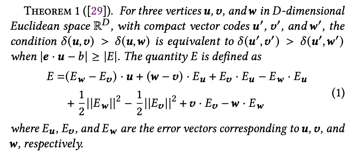
The paper extends this idea for compressed vectors through Theorem 1 (see the paper for the proof).

According to Theorem 1, when using compressed vectors u′, v′, w′, the distance comparison results remain consistent as long as the condition |e · u − b| ≥ |E| is satisfied.

Here, E denotes the compression error (see Theorem 1 for the precise definition). For each vector x, the error vector is defined as Eₓ = x − x′, where x′ is the compressed version of x.

From this, we can conclude that vector compression can be applied safely as long as the compression error is controlled.

Finding Compression Parameters

To determine suitable compression parameters, the paper conducts the following experiment:

Randomly sample 10,000 vectors from the dataset.
For each vector, find its 100 nearest neighbors, then select 2 of them to form a triple (u, v, w).
Compress each triple to obtain u′, v′, w′.
For each triple, compute |e · u − b| and |E|.
Choose the compression parameters that minimize vector size while satisfying |e · u − b| ≥ |E|.

Later in the paper, when introducing the proposed compression method Flash, several hyperparameters appear. However, the paper does not provide explicit guidance on how to set these hyperparameters to achieve sufficiently small |E|.

In practice, it is sufficient to understand that with properly chosen hyperparameters, |E| can be kept small enough that compressed vector search works effectively. Indeed, in the evaluation section of the paper, Flash achieves strong recall performance.

Flash: A New Vector Compression Method

The paper introduces a new compression method called Flash, which is inspired by PQ (Product Quantization), SQ (Scalar Quantization), and PCA—with PQ being the most heavily leveraged.

The core idea is to split high-dimensional vectors into multiple subspaces, and then process each subspace in parallel.

Modern CPUs can use multiple SIMD registers in parallel, and Flash exploits this capability:

Split a high-dimensional vector into several subspaces.
Assign each subspace to a corresponding SIMD register.
During distance computation, each register calculates the partial distance for its subspace in parallel.

ADT & SDT

Flash constructs two types of distance tables:

ADT (Asymmetric Distance Table)

Used during the Candidate Acquisition (CA) step.
Vectors are compressed with SQ (Scalar Quantization) so they can be directly loaded into registers.
Improves SIMD efficiency and minimizes register reads.

SDT (Symmetric Distance Table)

Used during the Neighbor Selection (NS) step.
Stored in cache for faster access.

Both ADT and SDT optimize the number of bits allocated when representing each compressed vector.

Hyperparameters

Flash has two key hyperparameters:

Number of Subspaces (MF)
Dimension of Principal Components (dF)

These parameters control the trade-off between indexing speed and search accuracy. However, they do not affect SIMD alignment or memory access patterns directly.

PCA

When compressing vectors by subspaces, it works best if variance is evenly distributed across dimensions. However, in real embedding data, information is often concentrated in certain dimensions.

To address this, Flash applies PCA (Principal Component Analysis):

Compute a centered matrix from the vector data.
Calculate the covariance matrix from the centered matrix.
Compute the eigenvalues (λ) of the covariance matrix.

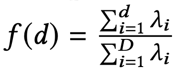
Then, define a function f(d) and set the principal component dimension dF as the minimum dimension such that f(d) ≥ α.

This way, Flash reduces the dimensionality of vectors while minimizing information loss.

Note: If you are unfamiliar with PCA, this part may be a bit difficult to follow. However, understanding PCA is not necessary for the rest of the discussion.

Subspace Division and Distance Table Compression

To maximize SIMD efficiency, Flash divides high-dimensional vectors into subspaces.

After applying PCA, the compressed vector is composed of sub-vectors.

Flash then constructs codebooks (similar to PQ) for each subspace i:

cᵢⱼ: centroid of the i-th subspace
K: number of centroids (codewords)

Each sub-vector uᵢ is mapped to its nearest centroid using the following rule:

As a result, one vector is represented by MF codewords. Since each codeword must represent K centroids, it requires log₂K bits.

ADT: Asymmetric Distance Table

For each input vector, Flash generates an ADT (Asymmetric Distance Table). The ADT stores the precomputed distances between the sub-vector uᵢ and all centroids in the corresponding codebook Cᵢ.

By precomputing the ADT, Flash can quickly calculate distances between the input vector and existing nodes during the Candidate Acquisition (CA) step.

However, to optimize for SIMD, the distance values cannot be stored as raw numbers. Instead, Flash applies Scalar Quantization (SQ) to quantize the distances as follows:

η(dist): quantized distance
Δ: quantization step size (Δ = distₘₐₓ − distₘᵢₙ)
H: number of bits allocated to represent the quantized distance

For example, if K = 16 and H = 8, the ADT requires a total of 128 bits, which fits perfectly into a single SIMD register.

During processing, the ADT exists as a one-dimensional array inside the register. Once input processing is complete, it is released from memory.

SDT: Symmetric Distance Table

During the Neighbor Selection (NS) step, Flash uses an SDT (Symmetric Distance Table) instead of ADT.

The SDT stores precomputed distance information between codewords within each subspace—i.e., the pairwise distances between centroids.

A total of MF SDTs are created (one per subspace).
Each SDT contains K × K distance values.
They are stored in cache as 2D arrays for fast access.

Access-Aware Memory Layout

In the standard HNSW indexing structure, each vector has a fixed-size neighbor list, and the vector’s position in memory is determined by its vertex ID. In other words, the offset is computed from the ID, and the algorithm accesses that location.

The problem is that neighbor vectors are too large to be stored contiguously with their IDs, which leads to random memory access.

Flash solves this by storing ID + codeword instead of the full vector. Each vertex’s neighbor list is structured as follows:

Neighbor IDs are stored in a fixed-size memory block.
Right next to them, the codewords of each neighbor are stored in sequence.

With this layout, distance computations during graph traversal can be performed using just the codewords—without fetching entire vectors. This eliminates random memory access, while also ensuring that the data is perfectly aligned for SIMD operations.

SIMD

In Flash, the ADT already stores quantized distance values for each subspace in SIMD registers. During distance computations, Flash leverages these SIMD registers as follows:

In a single operation, load B neighbor codewords into the SIMD register.
Each codeword acts as an index pointing to the corresponding partial distance in the ADT.
Use the SIMD shuffle operation to reorder the register values according to these indices.

Advantages of This Approach

Eliminates the need for branching.
Allows direct extraction of distance values from the ADT without additional memory accesses.
Extremely fast, since all operations occur within registers.

After that, the partial distances from each subspace are summed up to obtain the final distance. This summation is also performed using SIMD.

By using SIMD shuffle for ADT lookups and SIMD add for distance aggregation, Flash is not just about compressing data—it fundamentally redesigns the computation flow to align with SIMD execution.

HNSW + Flash

Flash is designed to integrate seamlessly into the existing HNSW framework.

The implementation process can be divided into three main phases: preprocessing → index construction → distance computation.

1. Preprocessing: PCA and Codebook Construction

First, the principal components are extracted from the dataset:

Sample a subset of the dataset.
Apply PCA to extract principal components.
For each subspace, construct a codebook.
Based on centroid distances, build the SDT (Symmetric Distance Table).

2. Index Construction: Codeword Conversion & ADT Setup

When constructing the index, each vector u undergoes the following process:

Compress u via PCA and split it into multiple sub-vectors uᵢ.
Each sub-vector is mapped to the closest centroid in its codebook Cᵢ.
This mapping generates codewords, with each codeword requiring log₂K bits.

At this stage, the ADT (Asymmetric Distance Table) is constructed as follows:

Compute distances between each uᵢ and the centroids in Cᵢ.
Quantize these distances using SQ (Scalar Quantization).
The resulting ADT is stored in SIMD registers and maintained until input processing is complete.

3. Distance Computation: Using ADT & SDT

During index construction, Flash performs two types of distance calculations:

Vector u ↔ Neighbor Batch distance computation → uses ADT.
Candidate ↔ Candidate distance computation → uses SDT.

The ADT is stored in a SIMD-friendly layout, enabling fast batch distance computations. The SDT, in turn, is used for efficient candidate-to-candidate comparisons.

4. Hyperparameter Settings

Flash introduces several hyperparameters:

MF: number of subspaces
dF: dimension of principal components
LF: number of bits per codeword
B: batch size

MF and dF are used to adjust compression error.
LF and B are determined by the size of SIMD registers.

Cost Analysis

(1) Candidate Acquisition (CA) Step

Original HNSW

Time complexity: O(R · log n)

R: maximum number of neighbors
log n: average search path length

At each hop, the algorithm must access neighbor vector data, leading to random memory accesses.

With Flash

Time complexity: O(log n)

Flash stores neighbor IDs + codewords in contiguous memory blocks, so full vectors don’t need to be loaded—distances can be computed directly from codewords.

This effectively eliminates random memory access.

Additionally, since vectors are compressed, the overall data size is smaller, which increases cache hit rates.

(2) Neighbor Selection (NS) Step

Original HNSW

For each candidate comparison, the vector data must be reloaded.
Memory access count: O(C), where C is the candidate set size.

With Flash

No vector accesses are required.
All distance information is precomputed and stored in the SDT (Symmetric Distance Table). Since the SDT is small enough to fit into L1 cache, once loaded, zero additional memory accesses are needed.

(3) SIMD-Based Distance Computation: Memory Load Count

Original HNSW

Load count: 32 · D / U

32 = number of bits in a float
D = vector dimension
U = SIMD register width (in bits)

With Flash

Load count: MF · H / U

MF = number of subspaces
H = number of bits per quantized distance per subspace

Example:
If D = 768, U = 128, MF = 16, H = 8,
→ SIMD load count is reduced by 192× compared to standard HNSW.

Evaluation

The paper sets the parameters as follows:

C (maximum number of candidates): 1024
R (maximum number of neighbors): 32

It compares standard HNSW against HNSW with PCA, SQ, PQ, and Flash-based vector encoding.

(1) Index Construction Time

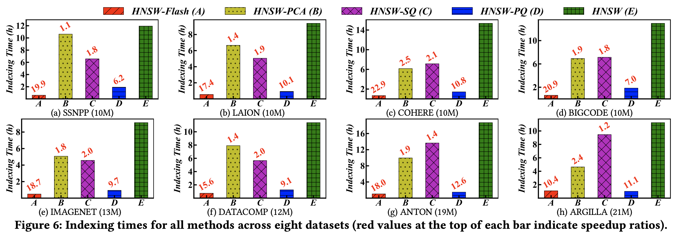
The index construction time includes both the indexing process and the preprocessing time required for encoding.

HNSW-Flash achieves 10–20× faster index construction compared to standard HNSW. It also significantly outperforms other compression methods.

(2) Index Size

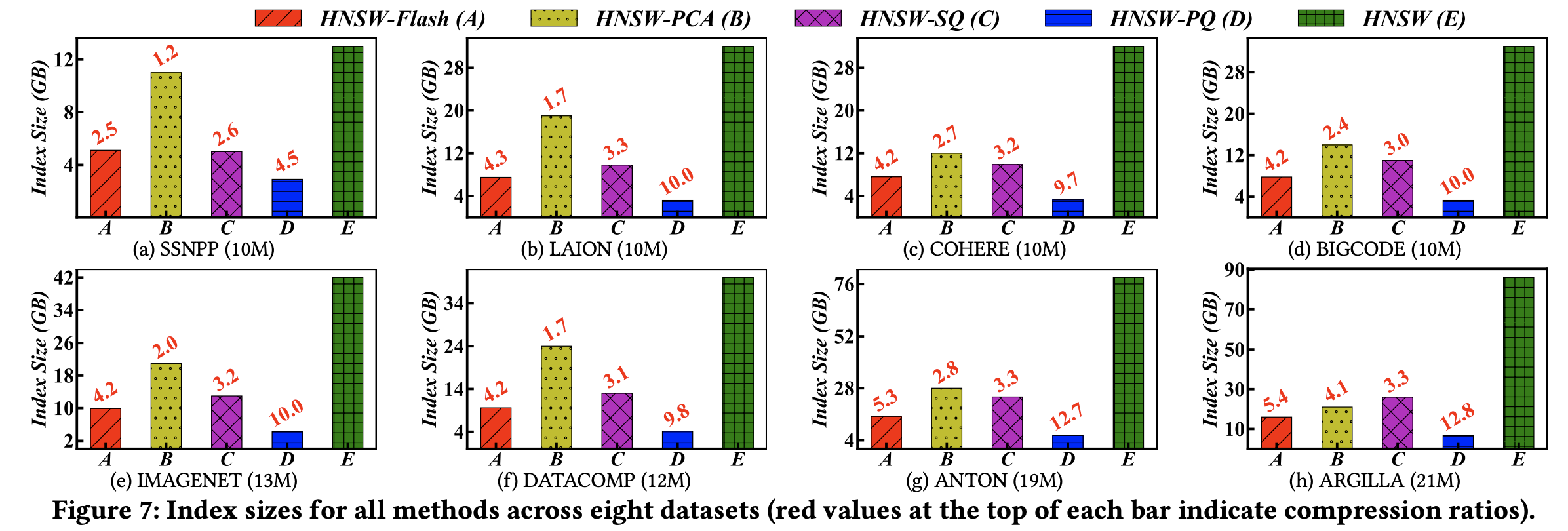
With Flash applied, the index size is reduced by approximately 2–5× compared to the uncompressed version.

(3) QPS – Recall

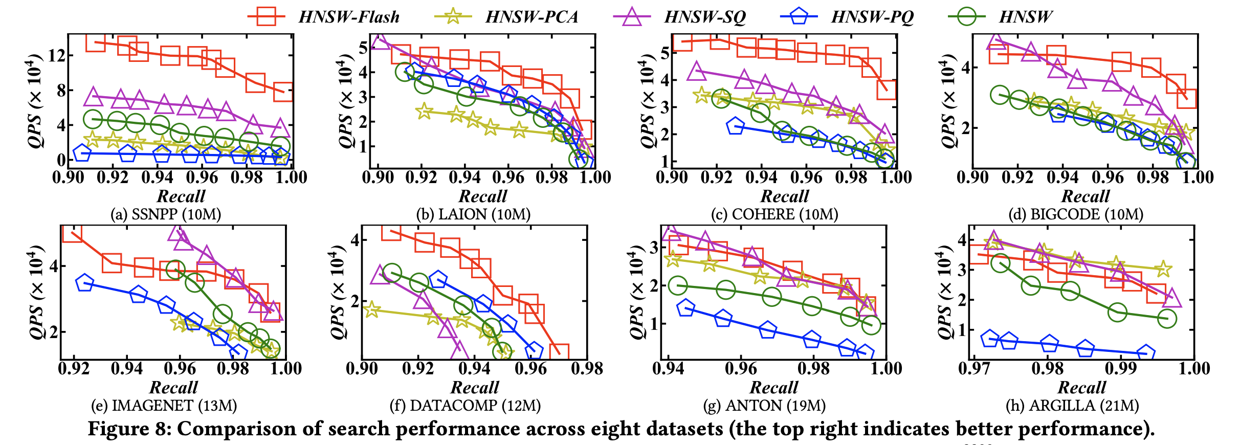
At the same recall level, Flash records a much higher QPS (queries per second) compared to other methods.

(4) Breakdown of Index Construction Time with Flash

When analyzing index construction under Flash, Coding Time accounts for about 10% of the total index construction time.

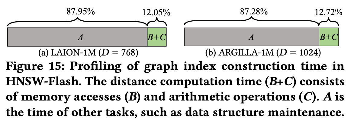
The previously identified bottleneck—distance computation + memory access—drops to only 12% of the total construction time after applying Flash.

(5) Hyperparameters

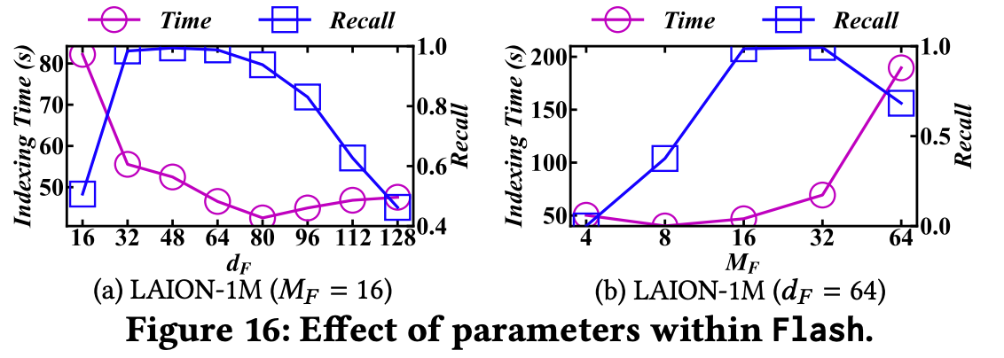
dF (dimension of principal components) and MF (number of subspaces) both influence indexing efficiency and index quality.

According to the evaluation, the optimal setting is: MF = 16, dF = 64

My Thoughts

Points to Consider Before Applying Flash in a Service

(1) Potential Performance Drop with Incremental Inserts into HNSW
Looking at the Flash implementation, PCA is applied to the entire dataset to reduce dimensionality and generate the basis vectors. These basis vectors are then used to compress all vectors.

Similarly, PQ (Product Quantization) is performed on the dataset to quantize subspaces of the vectors.

This approach is very suitable when building an HNSW index in batch mode.

However, if new vectors are incrementally inserted into an already-built HNSW index, they may not be properly compressed (leading to information loss). This is because PCA and PQ are optimized for the existing dataset.

As a result, if incremental insertions are frequent, recall performance could degrade.

(2) Overhead of PCA and PQ
Before inserting vectors into the index, Flash requires PCA and PQ preprocessing.

This preprocessing is not applied per vector but must be performed once over the entire dataset, which could be a heavy burden from an application perspective.

Impressions

Personally, I liked this paper because Flash can be applied without modifying the HNSW code itself. That makes it a practical approach many services could try.

I was also impressed that the proposed compression method (Flash) goes beyond simple compression—it is carefully designed to optimize SIMD operations by constructing ADTs and SDTs and using them effectively.

Despite this careful design, Flash is not difficult to understand (if you are already familiar with PCA and PQ), which makes it a very good algorithm in my opinion.

Moreover, I believe the ideas used in Flash could remain useful even beyond HNSW—applicable to future vector search algorithms as well. This is why I think it’s worth fully understanding this paper.

If you are working with vector search, I recommend considering Flash. The authors have also released an implementation of the method.

Reference

Accelerating Graph Indexing for ANNS on Modern CPUs

Flash Github